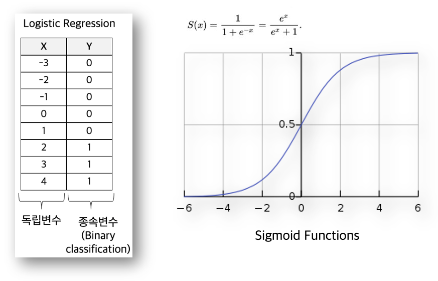
Logistic regression은 독립 변수의 선형 결합을 이용하여 사건의 발생 가능성을 예측하는데 사용되는 통계 기법입니다. 일반적인 선형회귀와 차이점은 종속 변수가 특정 분류로 나뉘는 특징이 있고, 결과가 1 또는 0으로 제한되는 이전 분류 (Binary Classification)입니다.
Logistic regression에서의 각 독립 변수의 계수를 log-odds를 구한된 Sigmoid함수를 적용하여 실제 데이터가 해당 class에서 속할 확률을 계산합니다. 즉, Logistics regression에서의 가설(Hypothesis)은 Sigmoid function입니다. Loss(손실, 오차)는 예측 모델이 실제의 값을 얼마나 잘 표현하는지 나타내는 함수로 binary_crossentropy를 사용하고 있습니다. 특정 데이터가 1 또는 0으로 분류하는 기준인 Classification thresold는 0.5 값을 사용합니다. 수학적인 증명을 위해서는 odds, logit 변환에 대한 설명이 필요하며, 참고 링크1과 링크2를 확인 부탁드립니다. Google Machine Learning Crash Course의 Logicstics regression Video 강의도 좋은 참고해주세요.
- Hypothesis (가설) : Sigmoid Function. (0, 1) 사이의 값을 표현합니다.
- Loss (손실, 비용, 오차) : binary_crossentropy. (데이터의 label이 1 or 0인 경우 binary_crossentropy, [0, 1] 또는 [1,0] 이면 categorical_crossentrpy 임)
- Classfication thresold: 0.5 (확률 값이 0.5 이상이면 1, 0.5 이하면 0)

Python Keras 로 logistics regression code
Python Keras code에는 기존 Linear regression code 에서 ① Data set 부분과 ② Activation 함수를 sigmoid를 변경, ③ loss를 binary_crossentropy로 변경해야 합니다. 만일 여러 개의 독립 변수(X)가 있다면 Model의 Layer 입력 값을 독립 변수의 개수 만큼 input_dim을 설정해 주면 됩니다.

Training Evaluation 및 Prediction 결과 확인
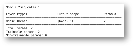
model.summary()를 통해서 Model을 확인하면, 기계 학습 Parameter 2개이고, Output shape은 1 dim인 model입니다
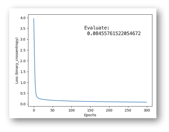
300회의 epochs 반복 학습 후 loss 값은 0.08로 매우 작은 값을 가지고 있습니다. epochs 200 이상에서는 loss값에 크게 변경이 없어 epochs 값은 200 이상이 적당한 것으로 보입니다.
원래 모델이 X < 2 인 경우에는 0 값, X ≥ 2 인 경우에는 1값으로 설정하는 계단 함수입니다. X=7인 경우에는 0.99 값으로 1 값으로 예측할 수 있고, X=-2 인 경우에는 0.005 값으로 Threshold 0.5 값 보다 적어 0 값으로 예측할 수 있습니다.

Logistic Regression Sample code
앞에서 설명한 Sample code는 GitHub에 올렸고, code는 아래와 같습니다. Sample code 출처는 https://www.edwith.org/pnu-deeplearning/lecture/57302/ 이며, 최신 Keras 버전에서 에러 나는 부분을 수정하고, Graph 생성 부분을 추가하였습니다.
#!/usr/bin/env python3
# -*- coding:utf-8 -*-

import numpy as np

from tensorflow.keras.models import Sequential
from tensorflow.keras.layers import Dense
from tensorflow.keras import optimizers

import matplotlib.pyplot as plt

# data set
x_data = np.array([-5, -4, -3, -2, -1, 0,1,2,3,4,5,6])
y_data = np.array([ 0,  0, 0,   0,  0, 0,0,1,1,1,1,1])

# model: linear regression input dense with dim =1
model = Sequential()
model.add(Dense(1, input_dim = 1, activation='sigmoid'))

# model compile:  SGD learning_rate of 0.01
sgd = optimizers.SGD(learning_rate = 0.01)
model.compile(loss='binary_crossentropy', optimizer=sgd)

# model fit
history = model.fit(x_data, y_data, epochs=300, batch_size=1, shuffle=False)

loss_and_metric = model.evaluate(x_data, y_data, batch_size=1)
print ('Evaluate:\n', loss_and_metric)

# prediction
print ('Predict:\n', model.predict([7, -2, -3, 2, 1]))

# print model summary
print ('Model summary:\n')
model.summary()

# 학습 정확성 값과 검증 정확성 값을 플롯팅 합니다.
#print(history.history)
plt.plot(history.history['loss'])
plt.ylabel('Loss (binary_crossentropy)')
plt.xlabel('Epochs')
plt.savefig('03_tran_result.png')
#plt.show()
관련 글:
[SW 개발/Data 분석 (RDB, NoSQL, Dataframe)] - Python Keras를 이용한 Linear regression 예측 (Sample code)
[SW 개발/Data 분석 (RDB, NoSQL, Dataframe)] - Python Pandas로 Excel과 CSV 파일 입출력 방법
[SW 개발/Python] - Python 정규식(Regular Expression) re 모듈 사용법 및 예제
댓글